Key Issue 4: Why Do Services Cluster In Settlements?

Determining The Optimal Number Of Clusters: three Must Know Methods

Determining the optimal number of clusters in a information gear up is a key issue in partition clustering, such as k-means clustering, which requires the user to specify the number of clusters chiliad to be generated.

Unfortunately, there is no definitive answer to this question. The optimal number of clusters is somehow subjective and depends on the method used for measuring similarities and the parameters used for partition.
A simple and popular solution consists of inspecting the dendrogram produced using hierarchical clustering to see if it suggests a particular number of clusters. Unfortunately, this arroyo is also subjective.

In this affiliate, nosotros'll describe different methods for determining the optimal number of clusters for grand-ways, k-medoids (PAM) and hierarchical clustering.

These methods include direct methods and statistical testing methods:

1. Straight methods: consists of optimizing a criterion, such as the inside cluster sums of squares or the boilerplate silhouette. The corresponding methods are named elbow and silhouette methods, respectively.
2. Statistical testing methods: consists of comparison testify confronting zip hypothesis. An example is the gap statistic.

In addition to elbow, silhouette and gap statistic methods, there are more than than 30 other indices and methods that accept been published for identifying the optimal number of clusters. We'll provide R codes for computing all these 30 indices in order to decide the best number of clusters using the "majority rule".

For each of these methods:

• We'll describe the basic idea and the algorithm
• We'll provide easy-o-use R codes with many examples for determining the optimal number of clusters and visualizing the output.

Contents:

• Elbow method
• Average silhouette method
• Gap statistic method
• Computing the number of clusters using R
  • Required R packages
  • Data preparation
  • fviz_nbclust() office: Elbow, Silhouhette and Gap statistic methods
  • NbClust() function: 30 indices for choosing the all-time number of clusters
• Summary
• References

Related Volume

Practical Guide to Cluster Analysis in R

Elbow method

Retrieve that, the basic idea behind sectionalisation methods, such as k-means clustering, is to define clusters such that the total intra-cluster variation [or total within-cluster sum of foursquare (WSS)] is minimized. The total WSS measures the compactness of the clustering and nosotros want information technology to be as small-scale every bit possible.

The Elbow method looks at the full WSS as a function of the number of clusters: Ane should choose a number of clusters so that adding another cluster doesn't improve much better the total WSS.

The optimal number of clusters can exist defined equally follow:

1. Compute clustering algorithm (e.g., k-ways clustering) for different values of chiliad. For instance, past varying k from 1 to 10 clusters.
2. For each thou, summate the total within-cluster sum of foursquare (wss).
3. Plot the bend of wss co-ordinate to the number of clusters one thousand.
4. The location of a curve (knee) in the plot is generally considered as an indicator of the appropriate number of clusters.

Notation that, the elbow method is sometimes ambiguous. An culling is the average silhouette method (Kaufman and Rousseeuw [1990]) which can be also used with any clustering approach.

Average silhouette method

The boilerplate silhouette arroyo we'll be described comprehensively in the chapter cluster validation statistics. Briefly, it measures the quality of a clustering. That is, it determines how well each object lies within its cluster. A loftier average silhouette width indicates a good clustering.

Average silhouette method computes the average silhouette of observations for different values of k. The optimal number of clusters thou is the one that maximize the average silhouette over a range of possible values for 1000 (Kaufman and Rousseeuw 1990).

The algorithm is similar to the elbow method and tin can be computed as follow:

1. Compute clustering algorithm (e.thou., k-means clustering) for dissimilar values of grand. For case, by varying k from one to 10 clusters.
2. For each thou, calculate the average silhouette of observations ( a v yard.s i fifty ).
3. Plot the bend of a v g.s i l according to the number of clusters g.
4. The location of the maximum is considered equally the appropriate number of clusters.

Gap statistic method

The gap statistic has been published by R. Tibshirani, G. Walther, and T. Hastie (Standford University, 2001). The approach tin can exist applied to whatsoever clustering method.

The gap statistic compares the total within intra-cluster variation for unlike values of k with their expected values under null reference distribution of the information. The estimate of the optimal clusters will be value that maximize the gap statistic (i.e, that yields the largest gap statistic). This means that the clustering structure is far abroad from the random uniform distribution of points.

The algorithm works as follow:

1. Cluster the observed data, varying the number of clusters from k = 1, …, k _{m a ten} , and compute the corresponding total within intra-cluster variation W _k .
2. Generate B reference information sets with a random uniform distribution. Cluster each of these reference data sets with varying number of clusters k = 1, …, k _{one thousand a x} , and compute the corresponding full within intra-cluster variation W _{k b} .
3. Compute the estimated gap statistic as the difference of the observed W _k value from its expected value W _{m b} nether the nix hypothesis: \(Gap(yard) = \frac{1}{B} \sum\limits_{b=i}^B log(W_{kb}^*) - log(W_k)\) . Compute too the standard deviation of the statistics.
4. Choose the number of clusters as the smallest value of one thousand such that the gap statistic is inside one standard departure of the gap at yard+one: Thousand a p(one thousand)≥G a p(k + 1)−south _{chiliad + one} .

Note that, using B = 500 gives quite precise results then that the gap plot is basically unchanged after an another run.

Computing the number of clusters using R

In this section, we'll draw two functions for determining the optimal number of clusters:

1. fviz_nbclust() function [in factoextra R package]: It can be used to compute the three dissimilar methods [elbow, silhouette and gap statistic] for whatever partitioning clustering methods [One thousand-ways, K-medoids (PAM), CLARA, HCUT]. Note that the hcut() part is bachelor only in factoextra package.It computes hierarchical clustering and cutting the tree in k pre-specified clusters.
2. NbClust() function [ in NbClust R packet] (Charrad et al. 2014): It provides xxx indices for determining the relevant number of clusters and proposes to users the best clustering scheme from the different results obtained by varying all combinations of number of clusters, distance measures, and clustering methods. It tin simultaneously computes all the indices and determine the number of clusters in a single function phone call.

Required R packages

We'll employ the following R packages:

• factoextra to determine the optimal number clusters for a given clustering methods and for information visualization.
• NbClust for computing about 30 methods at once, in order to find the optimal number of clusters.

To install the packages, type this:

                      pkgs <- c("factoextra",  "NbClust") install.packages(pkgs)                    

Load the packages as follow:

                      library(factoextra) library(NbClust)                    

Data preparation

We'll use the USArrests data as a demo information set. Nosotros start by standardizing the data to make variables comparable.

                      # Standardize the data df <- calibration(USArrests) head(df)                    

                      ##            Murder Assault UrbanPop     Rape ## Alabama    1.2426   0.783   -0.521 -0.00342 ## Alaska     0.5079   i.107   -1.212  two.48420 ## Arizona    0.0716   1.479    0.999  1.04288 ## Arkansas   0.2323   0.231   -1.074 -0.18492 ## California 0.2783   ane.263    1.759  2.06782 ## Colorado   0.0257   0.399    0.861  1.86497                    

fviz_nbclust() function: Elbow, Silhouhette and Gap statistic methods

The simplified format is as follow:

                      fviz_nbclust(x, FUNcluster, method = c("silhouette", "wss", "gap_stat"))                    

• x: numeric matrix or data frame
• FUNcluster: a sectionalisation function. Immune values include kmeans, pam, clara and hcut (for hierarchical clustering).
• method: the method to be used for determining the optimal number of clusters.

The R code below determine the optimal number of clusters for k-means clustering:

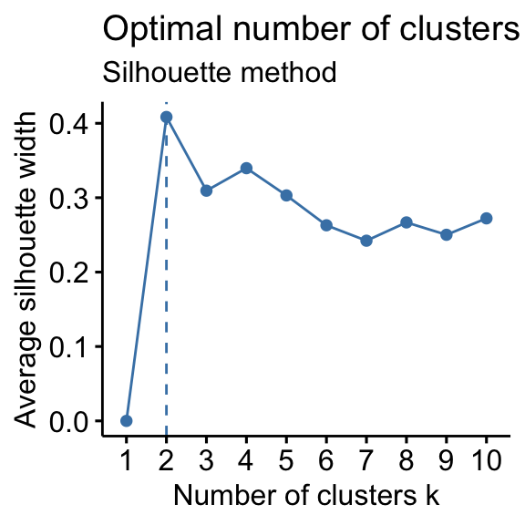
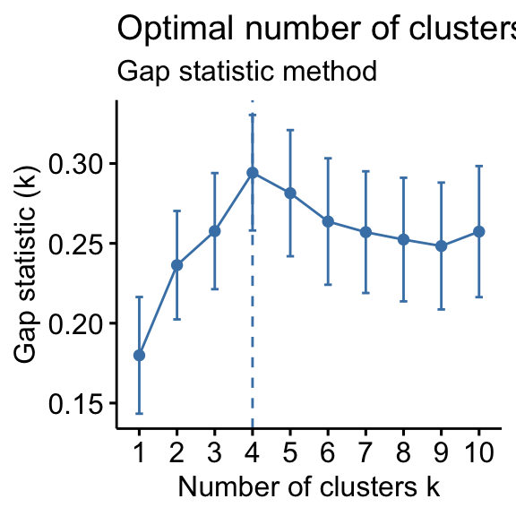
                      # Elbow method fviz_nbclust(df, kmeans, method = "wss") +     geom_vline(xintercept = four, linetype = 2)+   labs(subtitle = "Elbow method")  # Silhouette method fviz_nbclust(df, kmeans, method = "silhouette")+   labs(subtitle = "Silhouette method")  # Gap statistic # nboot = 50 to go on the function speedy.  # recommended value: nboot= 500 for your analysis. # Utilize verbose = FALSE to hibernate computing progression. set.seed(123) fviz_nbclust(df, kmeans, nstart = 25,  method = "gap_stat", nboot = fifty)+   labs(subtitle = "Gap statistic method")                    

                      ## Clustering k = 1,two,..., K.max (= x): .. done ## Bootstrapping, b = 1,2,..., B (= 50)  [one "." per sample]: ## .................................................. fifty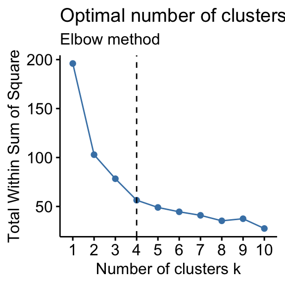                    

• Elbow method: 4 clusters solution suggested
• Silhouette method: 2 clusters solution suggested
• Gap statistic method: 4 clusters solution suggested

According to these observations, it's possible to define k = 4 as the optimal number of clusters in the data.

The disadvantage of elbow and average silhouette methods is that, they measure a global clustering characteristic but. A more sophisticated method is to utilise the gap statistic which provides a statistical process to formalize the elbow/silhouette heuristic in order to approximate the optimal number of clusters.

NbClust() function: 30 indices for choosing the best number of clusters

The simplified format of the function NbClust() is:

                      NbClust(information = Cipher, diss = NULL, altitude = "euclidean",         min.nc = 2, max.nc = xv, method = NULL)                    

• data: matrix
• diss: contrast matrix to be used. Past default, diss=NULL, but if it is replaced by a dissimilarity matrix, distance should exist "NULL"
• distance: the distance measure to be used to compute the dissimilarity matrix. Possible values include "euclidean", "manhattan" or "NULL".
• min.nc, max.nc: minimal and maximal number of clusters, respectively
• method: The cluster assay method to be used including "ward.D", "ward.D2", "single", "complete", "average", "kmeans" and more.

• To compute NbClust() for kmeans, use method = "kmeans".
• To compute NbClust() for hierarchical clustering, method should be 1 of c("ward.D", "ward.D2", "single", "complete", "average").

The R code below computes NbClust() for one thousand-means:

Here, there are contents hidden to non-premium members. Sign up now to read all of our premium contents and to be awarded a certificate of course completion.
Claim Your Membership At present

                      ## Among all indices:  ## =================== ## * two proposed  0 as the best number of clusters ## * 10 proposed  ii every bit the best number of clusters ## * 2 proposed  3 as the best number of clusters ## * 8 proposed  4 every bit the best number of clusters ## * 1 proposed  v as the all-time number of clusters ## * 1 proposed  8 as the best number of clusters ## * 2 proposed  10 as the best number of clusters ##  ## Determination ## ========================= ## * According to the majority rule, the best number of clusters is  ii .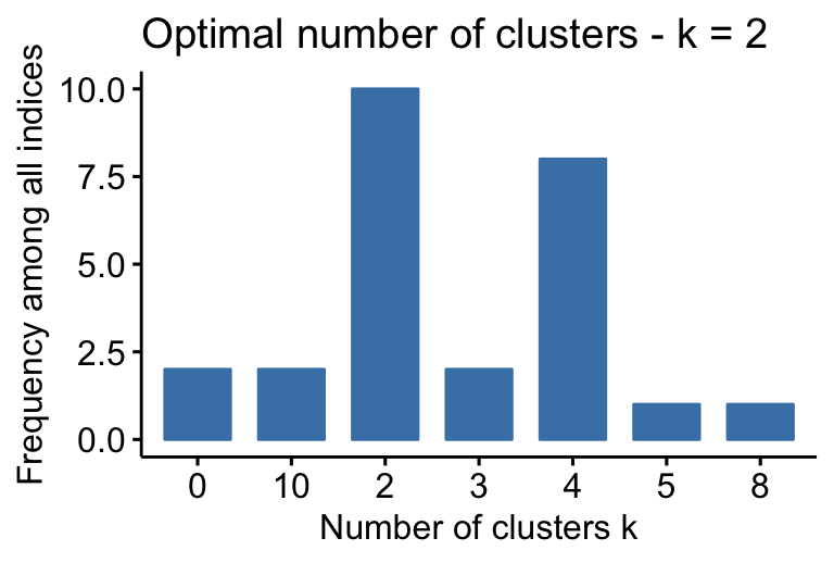                    

• ….
• 2 proposed 0 as the best number of clusters
• ten indices proposed 2 as the best number of clusters.
• ii proposed iii every bit the best number of clusters.
• viii proposed four as the best number of clusters.

According to the majority rule, the best number of clusters is two.

Summary

In this article, nosotros described dissimilar methods for choosing the optimal number of clusters in a data set up. These methods include the elbow, the silhouette and the gap statistic methods.

We demonstrated how to compute these methods using the R function fviz_nbclust() [in factoextra R package]. Additionally, we described the package NbClust(), which can be used to compute simultaneously many other indices and methods for determining the number of clusters.

Afterwards choosing the number of clusters m, the next pace is to perform partitioning clustering every bit described at: k-means clustering.

References

Charrad, Malika, Nadia Ghazzali, Véronique Boiteau, and Azam Niknafs. 2014. "NbClust: An R Parcel for Determining the Relevant Number of Clusters in a Information Set." Periodical of Statistical Software 61: 1–36. http://www.jstatsoft.org/v61/i06/paper.

Kaufman, Leonard, and Peter Rousseeuw. 1990. Finding Groups in Data: An Introduction to Cluster Analysis.

Recommended for you

This section contains all-time data science and cocky-development resources to help you on your path.

Back to Cluster Validation Essentials

Instructor

Source: https://www.datanovia.com/en/lessons/determining-the-optimal-number-of-clusters-3-must-know-methods/

Posted by: garciamanneve.blogspot.com

Share this post